Viewing Recent Stations

One of the endpoints accessed by the hakaiApi package is the stations endpoint. This endpoint provides metadata about stations, including their geographic coordinates. This information can be useful for visualizing the locations of stations on a map. In R we can either make static maps using ggplot2 or interactive maps using mapview to quickly visualize the locations of stations. We need to install the bcmaps package to get a base map of British Columbia as well as the sf package to handle spatial data and the ggplot2 and mapview packages for visualization.

library(hakaiApi)
library(ggplot2)
library(mapview)
library(bcmaps)
#> Loading required package: sf
#> Linking to GEOS 3.12.1, GDAL 3.8.4, PROJ 9.4.0; sf_use_s2() is TRUE
#> Support for Spatial objects (`sp`) was removed in {bcmaps} v2.0.0. Please use `sf` objects with {bcmaps}.
library(sf)

We first need to access the stations endpoint using the Client class from the hakaiApi package. We can then use the get_stations method to retrieve a data frame of stations. If you don’t have the sf package installed you will prompted to install that at this point.

hakai_client <- hakaiApi::Client$new("https://portal.hakai.org/api")
stations <- hakai_client$get_stations()

Because we want to plot the stations and some sensible basemap, we need to created a clipped polygon of British Columbia that contains all the stations. We can do this by creating a bounding box around the stations and then using the st_intersection function from the sf package to clip the BC polygon to that bounding box.

bc <- bcmaps::bc_bound_hres()
#> Creating directory to hold bcmaps data at /home/runner/.cache/R/bcmaps
#> Reading the data using the read_sf function from the sf package.

points_bbox <- st_bbox(stations) |> 
  st_as_sfc() |> 
  st_transform(st_crs(bc))
clipped_polygon <- st_intersection(bc, points_bbox)

Once we have the clipped polygon, we can plot the stations on top of it using ggplot2 or mapview. Here is an example of a static map using ggplot2:

ggplot() +
  geom_sf(data = clipped_polygon) +
  geom_sf(data = stations, aes(color = station_id), size = 3) +
  theme_minimal() +
  theme(legend.position = "bottom")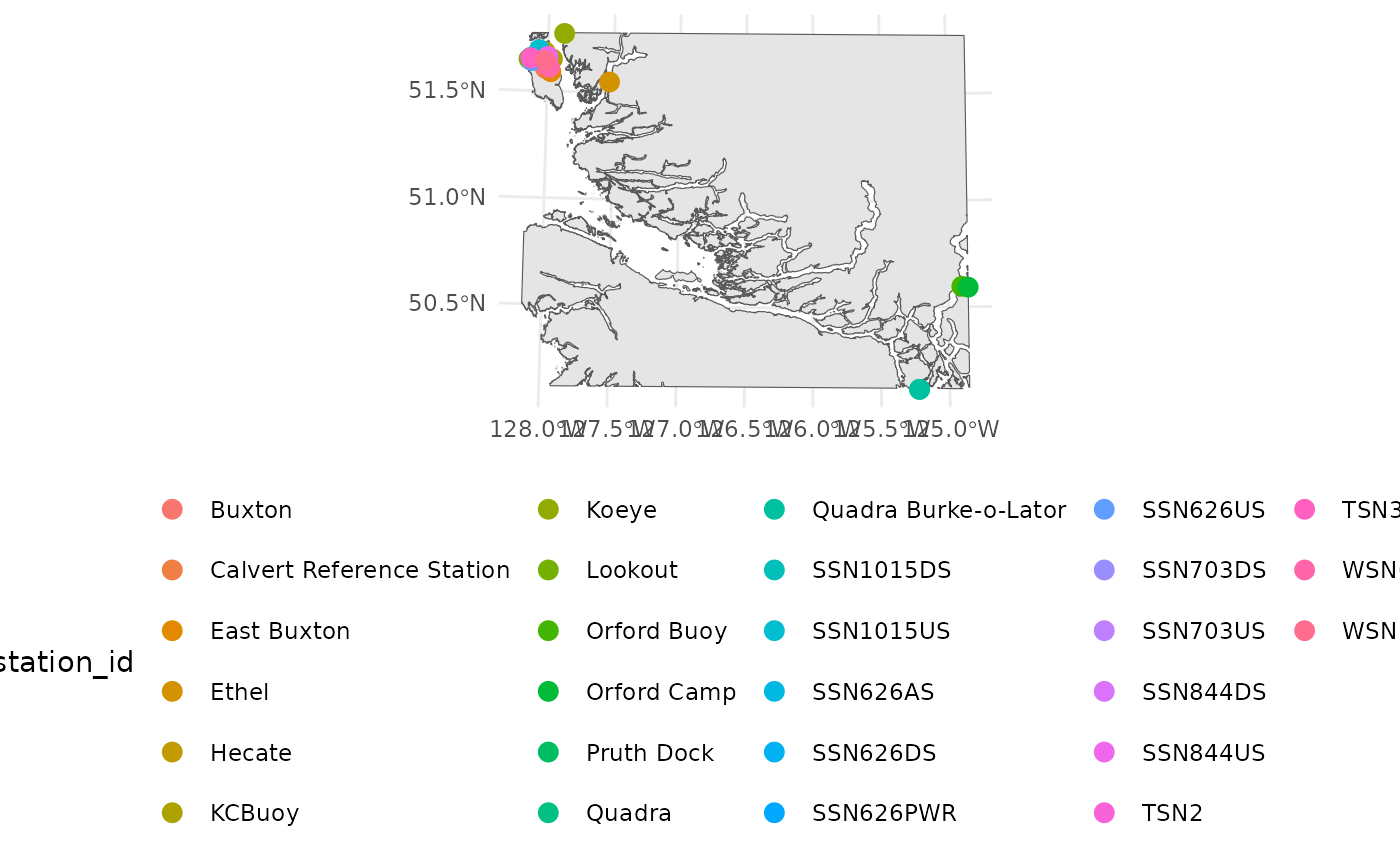

And here is an example of an interactive map using mapview:

mapview::mapview(stations)