
kelpbio fits Bayesian hierarchical models to estimate kelp biomass and carbon from field measurements.
Installation
Install the pre-built binary from the Hakai R-universe (macOS and Windows):
install.packages(
  "kelpbio",
  repos = c("https://hakaiinstitute.r-universe.dev", getOption("repos"))
)
Install from source (Linux, or to build from GitHub):
# install.packages("pak")
pak::pak("HakaiInstitute/kelpbio")
Source builds require a C++ toolchain:
- Linux:
sudo apt install build-essential - Windows: Rtools
- macOS:
xcode-select --install
Usage
kelpbio fits each biomass component with its own kb_fit_*() function. The allometric weight model relates wet weight to sub-bulb diameter, with random effects for site and site-by-year.
The model is fitted to a data frame of diameter, weight, site, and year. A small simulated dataset is included with the package:
library(kelpbio)

head(data_weight_sim_nereo)
#> # A tibble: 6 × 4
#>   diameter weight site  year
#>      <dbl>  <dbl> <fct> <fct>
#> 1     53.8  0.412 site1 2019
#> 2     38.2  0.183 site1 2019
#> 3     25.2  0.059 site1 2019
#> 4     54.5  0.523 site1 2019
#> 5     25.6  0.06  site1 2019
#> 6     49.5  0.411 site1 2019
Fit the model with kb_fit_weight_nereo():
fit <- kb_fit_weight_nereo(data_weight_sim_nereo, seed = 1)Fitting compiles and samples the Stan model, so a pre-fit model on this dataset is included with the package for quick exploration:
fit <- fit_weight_sim_nereoCheck convergence with glance() and summarise the model terms with tidy():
glance(fit)
#> # A tibble: 1 × 8
#>       n     K nchains niters nthin   ess  rhat converged
#>   <int> <int>   <int>  <dbl> <int> <dbl> <dbl> <lgl>
#> 1   234    10       2    400     1  201.  1.03 TRUE

tidy(fit)
#> # A tibble: 7 × 4
#>   term          estimate   lower  upper
#>   <chr>            <dbl>   <dbl>  <dbl>
#> 1 bWeight        -1.47   -1.66   -1.24
#> 2 bDiameter       2.5     2.28    2.74
#> 3 bDiameter2      0.0749 -0.156   0.313
#> 4 sSite           0.27    0.176   0.459
#> 5 sSiteDiameter   0.313   0.169   0.62
#> 6 sSiteYear       0.0962  0.0521  0.149
#> 7 sWeight         0.161   0.141   0.185
Predict the weight-diameter curve for each site with kb_predict_weight_by() and plot it with kb_plot_predictions():
kb_predict_weight_by(fit, by = "site") |>
  kb_plot_predictions()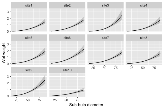
Predict weight at new diameters with kb_predict_weight(). It returns a table with a point estimate and conf_level compatibility limits for each row:
new_data <- data.frame(diameter = c(20, 35, 50, 65, 80), site = "site1")

set.seed(1)
kb_predict_weight(fit, new_data)
#> <kb_predictions> predictor: diameter | response: weight | by: site
#> # A tibble: 5 × 5
#>   diameter site  estimate  lower  upper
#>      <dbl> <chr>    <dbl>  <dbl>  <dbl>
#> 1       20 site1   0.0302 0.0229 0.0393
#> 2       35 site1   0.126  0.0975 0.162
#> 3       50 site1   0.319  0.242  0.421
#> 4       65 site1   0.647  0.49   0.85
#> 5       80 site1   1.12   0.842  1.52
The fitted object exposes the standard rstantools generics (posterior_predict(), log_lik(), and others), so it composes directly with bayesplot and loo.
Citation
If you use kelpbio in your work, please cite it. Use citation() to get a formatted citation and BibTeX entry:
citation("kelpbio")
#> To cite kelpbio in publications use:
#>
#>   Dalgarno S (2026). _kelpbio: Bayesian Kelp Biomass Estimation_. R
#>   package version 0.0.0.9000,
#>   <https://github.com/HakaiInstitute/kelpbio>.
#>
#> A BibTeX entry for LaTeX users is
#>
#>   @Manual{,
#>     title = {kelpbio: Bayesian Kelp Biomass Estimation},
#>     author = {Seb Dalgarno},
#>     year = {2026},
#>     note = {R package version 0.0.0.9000},
#>     url = {https://github.com/HakaiInstitute/kelpbio},
#>   }