
kelpbio fits Bayesian hierarchical Stan models to estimate kelp biomass from field measurements. This article walks through the allometric weight model for Nereocystis luetkeana, which relates wet weight to sub-bulb diameter with random effects for site and site-by-year. Further biomass components (plant size distribution, density, and wet-to-dry and carbon tissue conversions) are in development.
Under the hood, models are fitted with rstan. The Stan code is pre-compiled when the package is installed, so no separate Stan installation is required.
Providing data
The weight model is fitted to a data frame with a numeric
diameter, a numeric weight, and
site and year grouping factors. A small
simulated dataset is included with the package:
data_weight_sim_nereo
#> # A tibble: 234 × 4
#>    diameter weight site  year
#>       <dbl>  <dbl> <fct> <fct>
#>  1     53.8  0.412 site1 2019
#>  2     38.2  0.183 site1 2019
#>  3     25.2  0.059 site1 2019
#>  4     54.5  0.523 site1 2019
#>  5     25.6  0.06  site1 2019
#>  6     49.5  0.411 site1 2019
#>  7     63.7  0.693 site2 2019
#>  8     32.6  0.144 site2 2019
#>  9     44.5  0.166 site2 2019
#> 10     58    0.457 site2 2019
#> # ℹ 224 more rows
kb_check_data_weight_nereo() confirms the data are in
the expected format, returning the data invisibly if the checks pass and
raising an informative error otherwise:
kb_check_data_weight_nereo(data_weight_sim_nereo)Fitting the model
kb_fit_weight_nereo() fits the model. Set
progress = "none" to silence the sampler’s console output,
and seed for a reproducible fit.
fit <- kb_fit_weight_nereo(
  data_weight_sim_nereo,
  chains = 2,
  niters = 400,
  seed = 42
)
The short run above keeps the example quick; for a real analysis use
the defaults (chains = 4, niters = 1000) or
more.
Checking convergence
glance() returns a one-row summary of the fit, including
the sampler settings and the convergence diagnostics.
converged is TRUE when the split R-hat is
below its threshold (1.05 by default) and the effective sample size is
adequate.
glance(fit)
#> # A tibble: 1 × 8
#>       n     K nchains niters nthin   ess  rhat converged
#>   <int> <int>   <int>  <dbl> <int> <dbl> <dbl> <lgl>
#> 1   234    10       2    400     1  201.  1.03 TRUE
Summarising the fit
tidy() returns the model terms with a point estimate and
compatibility limits. The intercept and slopes describe the allometric
relationship on the log scale; the s-prefixed terms are the
random-effect standard deviations.
tidy(fit)
#> # A tibble: 7 × 4
#>   term          estimate   lower  upper
#>   <chr>            <dbl>   <dbl>  <dbl>
#> 1 bWeight        -1.47   -1.66   -1.24
#> 2 bDiameter       2.5     2.28    2.74
#> 3 bDiameter2      0.0749 -0.156   0.313
#> 4 sSite           0.27    0.176   0.459
#> 5 sSiteDiameter   0.313   0.169   0.62
#> 6 sSiteYear       0.0962  0.0521  0.149
#> 7 sWeight         0.161   0.141   0.185
Priors
kb_priors_weight_nereo() returns the default priors,
which are weakly informative on the model’s centered log scale.
kb_priors_weight_nereo()
#> $intercept
#> normal(mean = 0, sd = 2)
#>
#> $diameter
#> normal(mean = 2, sd = 1)
#>
#> $diameter2
#> normal(mean = 0, sd = 0.5)
#>
#> $sd_site
#> exponential(rate = 1)
#>
#> $sd_site_diameter
#> exponential(rate = 1)
#>
#> $sd_site_year
#> exponential(rate = 1)
#>
#> $sd_residual
#> exponential(rate = 1)
Adjust a prior by replacing an element with
kb_prior_normal() or kb_prior_exponential()
and passing the result to the priors argument of
kb_fit_weight_nereo():
priors <- kb_priors_weight_nereo()
priors$sd_site <- kb_prior_exponential(2)
fit <- kb_fit_weight_nereo(data_weight_sim_nereo, priors = priors, seed = 1)
Predictions
kb_predict_weight_by() summarises the fitted
weight-diameter curve over a generated diameter sequence, one curve per
group named in by. Pass the result to
kb_plot_predictions() to plot the curve with its
compatibility band:
kb_predict_weight_by(fit, by = "site") |>
  kb_plot_predictions()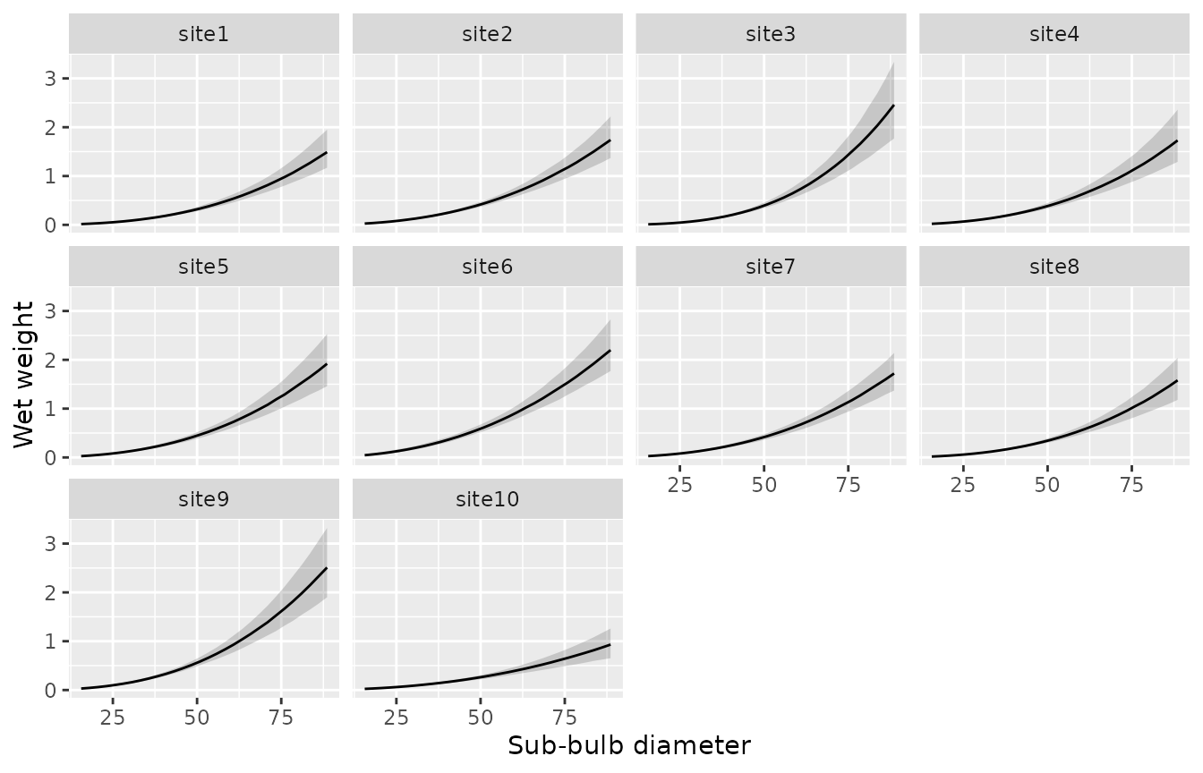
kb_predict_weight() instead predicts at the rows of a
supplied data frame, returning a point estimate and compatibility limits
for each row:
new_data <- data.frame(diameter = c(20, 35, 50, 65, 80), site = "site1")
kb_predict_weight(fit, new_data)
#> <kb_predictions> predictor: diameter | response: weight | by: site
#> # A tibble: 5 × 5
#>   diameter site  estimate  lower  upper
#>      <dbl> <chr>    <dbl>  <dbl>  <dbl>
#> 1       20 site1   0.0302 0.0233 0.0396
#> 2       35 site1   0.125  0.0992 0.155
#> 3       50 site1   0.321  0.25   0.405
#> 4       65 site1   0.647  0.501  0.857
#> 5       80 site1   1.12   0.86   1.51
Standard Bayesian tooling
The fitted object exposes the rstantools generics, so it
composes directly with bayesplot and loo. A
posterior-predictive check uses the stored yrep via
posterior_predict():
bayesplot::ppc_dens_overlay(
  y = fit$data$weight,
  yrep = posterior_predict(fit)
)
Leave-one-out cross-validation uses the pointwise
log_lik():